Raman spectroscopy in graphene and nanoribbons

Abstract

Raman spectroscopy in bulk graphene and nanoribbons are reviewed. First, a short introduction of graphene crystal structure and phonon dispersion is given. First-order and the double resonance Raman scattering mechanism in graphene are discussed to understand the most prominent Raman peaks. Raman in bulk graphene is discussed for numbers of layers with different stacking and substrate effects. Finally, we try to distinguish the zigzag and armchair type of graphene edges and the differences of Raman signal in nanoribbon and bulk graphene are discussed.

• Introduction

Graphene is a remarkable, two-dimensional material that has a number of unique electronic properties arising from a combination of its zero-gap linear dispersion, high carrier mobility, and high thermal conductivity. These electronic properties make graphene a leading contender to replace Si-based or III-V materials-based devices for high-frequency FET,¹ post-CMOS nanoelectronic devices,^2,3 and for use in even more futuristic devices based on photonics,⁴ spintronics^5,6 and quantum computing.⁷ Graphene’s combination of low mass and high mean free path leads to very high electronic mobility, with a record value of 230,000 cm²/V-sec for suspended graphene sheets.⁸

Crystal structure of graphene

Graphene is a two-dimensional (2D) planar structure based on a unit cell containing two carbon atoms A and B, as shown in Fig. 1. The structure can be seen as a triangular lattice composed by two vectors a1, a2 with a basis of two atoms per unit cell.

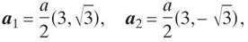
Where is the lattice constant of monolayer graphene. Likewise, the unit cell in reciprocal space is shown in Fig. 1 and is described by the unit vectors b1 and b2 of the reciprocal lattice given by

corresponding to a lattice of length in reciprocal space. The unit vectors b1 and b2 of the reciprocal hexagonal lattice are rotated by 30° from the unit vectors a1 and a2 in real space, respectively. The three high symmetry points of the Brillouin zone, Γ , K and M are the center, the corner, and the center of the edge of the hexagon, respectively. Other high symmetry points or lines are along ΓK (named T), KM (named T’) and ΓM (named Σ).

In monolayer graphene, three of the electrons form σ bonds which hybridize in a configuration, and the fourth electron of the carbon atom forms the orbital, which is perpendicular to the graphene plane, and makes π covalent bonds. Of particular importance for the physics of graphene are the two points K and K’ at the corners of the graphene Brillouin zone (BZ).

Fig. 1. Graphene honeycomb lattice and its Brillouin zone. Left: a₁ and a₂ are the lattice unit vectors, and δ_i, i=1,2,3 are the nearest-neighbor vectors. Right: The Dirac cones are located at the K and K’ points.

Phonon dispersion in graphene

The phonon dispersion of graphite plays a key role in interpreting its Raman spectra. In graphene there are 2 atoms per unit cell thus six phonon dispersion modes as seen in Fig. 2 out of which three are acoustic (A) and three are optical (O) phonon modes. For the three acoustic and three optical phonon modes, one is an out-of plane (oT) phonon mode and the other two are in-plane modes, one longitudinal (L) and the other one transverse (iTO). Thus, starting from the highest energy at the Γ point in the Brillouin zone the various phonon modes are labeled as LO, iTO, oTO, LA, iTA and oTA as shown in Fig. 2.

The optical phonons in the zone-center (Γ) and zone edge (K and K’) region are of particular interest, since they are accessible by Raman spectroscopy. The Γ point optical phonons are doubly degenerate with E2g symmetry for unperturbed graphene. The vibrations correspond to the rigid relative displacement of the A and B sub-lattices. This phonon mode is Raman active and responsible for the Raman G mode in graphene. The LO phonon branch near but away from the Γ point is not Raman active in a one- phonon process in defect free graphene, given that it has finite wave vector. However, in the presence of defects, it can be activated. Like the LO phonons around the Γ point, the TO phonon branch around the zone edge is accessible by a two-phonon Raman process, which gives rise to the G’ (also named 2D) mode.

Fig. 2. Calculated phonon dispersion relation of graphene showing the LO, iTO, oTO, LA, iTA, and oTA phonon branches.⁹

• Raman scattering mechanism in graphene

The most prominent features in the Raman spectra of monolayer graphene are the so-called G band appearing at 1582 cm⁻¹ (graphite) and the G’ band at about 2700 cm⁻¹ using laser excitation at 2.41 eV. In the case of a disordered sample or at the edge of a graphene sample, we can also see the so-called disorder-induced D-band, at about half of the frequency of the G band (around 1350 cm⁻¹ using laser excitation at 2.41 eV).

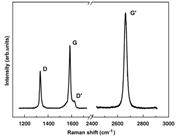
Fig. 3. Raman spectrum of a graphene edge, showing the main Raman features, the D, G and G’ bands taken with a laser excitation energy of 2.41 eV.

The G-band (for graphite) in the first-order Raman spectrum, corresponds to the optical mode vibration of two neighboring carbon atoms on a sp2-hybridized graphene layer. There is a tangential stretching of the σ bonds along the plane giving rise to the Raman G peak, which is one phonon intra-valley scattering process at the Γ point.

The double-resonance (DR) process shown in the center and right side of Fig. 4 begins with an electron of wave-vector k around K absorbing a photon of energy E_laser. The electron is inelastically scattered by a phonon or a defect of wavevector q and energy E_phonon to a point belonging to a circle around the K point, with wavevector k+q. The electron is then scattered back to a k state, and emits a photon by recombining with a hole at a k state. In the case of the D band, the two scattering processes consist of one elastic scattering event by defects of the crystal and one inelastic scattering event by emitting or absorbing a phonon, as shown in Fig. 4. In the case of the G’-band, both processes are inelastic scattering events and two phonons are involved.

The triple-resonance process can occur by both scattering of electrons and holes and the recombination happens at the inequivalent K’ point with respect to K point which generates the photon.

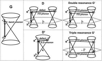
Fig. 4. (Left) First-order G-band process and (Center) one-phonon second-order DR process for the D-band (intervalley process) (top) and for the D-band (intravalley process) (bottom) and (Right) two-phonon second-order resonance Raman spectral processes (top) for the double resonance G process, and (bottom) for the triple resonance G band process (TR) for monolayer graphene. For one-phonon, second-order transitions, one of the two scattering events is an elastic scattering event. Resonance points are shown as open circles near the K point (left) and the K point (right).¹⁰

• Raman studies of the number of graphene layers and stacking orders

The G’ features like position, line width and intensity are dispersive with the number of layers ‘n’ of the graphene layer, as shown in Fig. 5. This is attributed to the evolution of the bands of the mono-layer, bi-layer and few-layer graphene structures. These dependences can be used to characterize the number of graphene layers ‘n’ in few layer graphene samples.

The G’ band for 1-LG at room temperature exhibits a single Lorentzian feature with a full width at half maximum (FWHM) of ∼24 cm⁻¹. For bilayer graphene with Bernal AB layer stacking, both the electronic and phonon bands split into two components. Four different DR processes¹¹ can happen in bilayer case. Thus Raman spectra of a 2-LG sample with AB stacking can be fitted with four Lorentzians, each with a FWHM of∼24 cm⁻¹. Using group theory analysis for a trilayer graphene, the number of allowed Raman peaks in the G’ band is fifteen. Due to the small energy separations of many of these fifteen transitions, experimentally it is found that the lineshape can be fitted with less peaks and the minimum number necessary to correctly fit the G’ is six. The high frequency side of the G’ band comes to dominate starting from 4-LG to HOPG. The G’ band is a convolution of peaks along the entire k_z axis.

Fig. 5. The measured G’ Raman band with 2.41 eV laser energy for (a) 1-LG, (b) 2-LG, (c) 3-LG, (d) 4-LG, (e) HOPG and (f) turbostratic graphite. The splitting of the G’ Raman band opens up in going from mono- to three-layer graphene and then closes up in going from 4-LG to HOPG.¹⁰

The identification of the number of layers by Raman spectroscopy is well established only for graphene samples with AB Bernal stacking. In the case of randomly rotation stacking like turbostratic graphite, Raman shows a G’ band that is a single Lorentzian as in monolayer graphene but with a larger FWHM OF ~45-60 cm^-1 and much smaller I_G’/I_G. This is due to the absence of an interlayer interaction between the graphene planes.

Recently, Intravalley R’ peak centered at∼1625 cm^-1 is observed in randomly produced bilayer graphene due to a rotational-induced intervalley DR mechanism.¹² Its properties depend on the mismatch rotation angle and can be used as an optical signature for superlattices in bilayer graphene.

• Substrate effect

Clear understanding of the substrate effect is important for the potential device fabrication of graphene. Micromechanically cleaved monolayer graphene on standard SiO₂ (300 nm)/Si, single crystal quartz, Si, glass, PDMS, and NiFe has been studied by Raman spectroscopy. It was found that G peak and G’ peak position and their FWHM have very small difference. The interaction between micromechanically cleaved graphene sheets and different substrates is not strong enough to affect the graphene sheets. G-band is made up of the long-wavelength optical phonons (TO and LO), and the out of plane vibrations in graphene are not coupled to this in-plane vibration. However, Raman of epitaxial graphene on SiC shows a big blueshift, which might due to strain effect and doping from substrate.

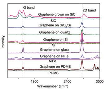
Fig. 6. The Raman spectra of monolayer graphene on different substrates as well that of epitaxial monolayer graphene on SiC.¹³

• Graphene edges

Graphene edges are of particular interest, since their chirality determines the electronic properties. The edge is either formed by carbon atoms arranged in the zigzag or armchair configuration as shown in Fig. 7. Zigzag edges are composed of carbon atoms that all belong to one and the same sublattice, whereas the armchair edge contains carbon atoms from either sublattice. For a zigzag edge the momentum can only be transferred in a direction d_z which does not allow the electron to return to the original valley in reciprocal space as shown in Fig. 7. Thus zigzag edges do not produce D peak in Raman spectroscopy. In graphene with perfect edges, if two edges form an angle of 120°, they should be the same. In contrast, an angle of 90 or 150° implies a change. In order to confirm this theory, Casiraghi¹⁴ carried out a detailed Raman investigation of graphene flakes with well-defined edges oriented at different crystallographic directions. The D to G ratio at the edge is never null due to some disorder at the edges.

Fig. 7. Raman double resonance mechanism in graphene and at the edge. (a) Atomic structure of the edge with armchair (blue) and zigzag (red) chirality. (b) Double resonance mechanism of the defect induced D peak. (c) First Brillouin zone of graphene and the double resonance mechanism in top view.¹⁵

By using carbo-thermal of SiO2 to SiO, Krauss¹⁵ able to make hexagonal holes with pure graphene zigzag edges. G peak appeared in both cases of round holes with mixture of zigzag and armchair edges and hexagonal holes with pure edge, while higher D peak intensity was shown in the vicinity of round holes. To rule out the random case, this was confirmed by statistic data.

Fig. 8. AFM images and Raman maps of graphene flakes containing round or hexagonal (top or bottom panels, respectively) holes. (a and d): AFM images of the round and hexagonal holes. (b and e) Intensity map of the Raman G peak. The G peak intensity is uniform across each flake except at the locations of the holes. These holes appear black (no graphene). The region where the AFM image was taken has been demarcated by a square. (c and f) Intensity map of the disorder-induced D peak. The D peak intensity is high in the vicinity of round holes (c). On the contrary, the D peak intensity is not enhanced near the hexagonal holes in (f).¹⁵

• Graphene nanoribbons

Comparing to bulk graphene material, graphene nanoribbons (GNRs) are becoming more interested in transistors applications and quantum confinement study. GNRs have been predicted to behave as a semiconductor with a bandgap which is determined by ribbon width and chirality. A ribbon with zigzag configuration on either edge has an almost flat energy band at the Dirac point giving rise to a large peak in the density of states. The charge density for these states is strongly localized on the zigzag edge sites. Nanoscale spintronic devices have been dreamed up to utilize such unique features. Armchair devices are particularly suitable candidates for spin quantum bits.

Optical characterization of newly emerging properties of GNRs has been rare. In particular, Raman spectroscopy has not been systematically investigated on GNRs. As results shown in graphene edge studying, we can expect the D peak will show up in the nanoribbons with disorder edges. Ryu¹⁶ found the G peak became lower and broader as the width decreased as shown in Fig. 9. Disparity was shown in G’ peak for nanoribbons with one monolayer and bilayer graphene, which can be used to distinguish the layer numbers of nanoribbons. The change in G peak does not surprise us since its intensity is proportional to the number of sp2 bonds. Since the laser spot (can be as small as 400 nm) are much bigger than the width of nanoribbons, the smaller the width the lesser area of graphene was detected in Raman.

Fig. 9. Raman spectra of GNR sets with different ribbon width at 632.8 nm excited energy. The bands at 1450 and 1650 cm^-1 are due to underlying Si and a plasma line of the excitation laser, respectively.¹⁶

Recently, a splitting of G^– at 1583 cm^-1 and G⁺ at 1594 cm^-1 was observed for H-terminated Z-GNRs, and a model was proposed to explain the dependence of I(G^–)/I(G⁺) on nanoribbon width.¹⁷ An individual Z-GNR has two spate portions: one is the edge-states affected portion (marked with red in Fig. 10.), contributing to G^– (softened E_2g-modeG); the other is the center portion (marked with blue in Fig. 10.), contributing to G⁺ (intrinsic E_2g-mode G⁺). When the nanoribbon width decreased, edge portion kept unchanged but central portion decreased, which decreased the I(G^–)/I(G⁺) as shown in Fig. 10.

Fig. 10. Width dependence of the relative intensity G^–/G⁺. (A) AFM images of GNRs with nearly perfect zigzag edge at different widths after nanopads removing. (B) Raman spectra for these Z-GNRs at different widths. (C) Fitted width dependence of the relative intensity G^–/G⁺. (D) Schematic of two-component Z-GNR: edge affected part (softened E_2g-mode G^–, as shown in red) and perfect bulk part (intrinsic E_2g-mode G⁺, as shown in blue).¹⁷

• Summary

Raman spectroscopy has been established as a very versatile characterization tool not just to identify layer number but also towards measurement of defectivity, substrate effects and edge effects. The understanding of these properties is highly essential for the study of graphene for future carbon-based devices. While Raman spectroscopy has low spatial resolution limited by optical system when applied to characterization of graphene nanoribbons. Combining with other technique like inelastic electron tunneling spectroscopy can reveal more details on phonon modes thus get a better understanding of electronic properties of graphene nanoribbons.

• Reference

1.    Lin, Y.-M. et al. 100-GHz transistors from wafer-scale epitaxial graphene. Science (New York, N.Y.)
327, 662 (2010).

2.    Banerjee, B.S.K. et al. Graphene for CMOS and Beyond CMOS Applications. Proceedings of the IEEE
98, (2010).

3.    Novoselov, K.S. et al. Electric field effect in atomically thin carbon films. Science (New York, N.Y.)
306, 666-9 (2004).

4.    Bonaccorso, F., Sun, Z., Hasan, T. & Ferrari, a. C. Graphene photonics and optoelectronics. Nature Photonics
4, 611-622 (2010).

5.    Son, Y.-W., Cohen, M.L. & Louie, S.G. Half-metallic graphene nanoribbons. Nature
444, 347-9 (2006).

6.    Tombros, N., Jozsa, C., Popinciuc, M., Jonkman, H.T. & van Wees, B.J. Electronic spin transport and spin precession in single graphene layers at room temperature. Nature
448, 571-4 (2007).

7.    Cortijo, A., Guinea, F. & Vozmediano, M.A.H. Geometrical and topological aspects of graphene and related materials. Arxiv preprint arXiv:1112.2054 1-34 (2011).at <http://arxiv.org/abs/1112.2054&gt;

8.    Bolotin, K. et al. Ultrahigh electron mobility in suspended graphene. Solid State Communications
146, 351-355 (2008).

9.    Dresselhaus, M.S., Jorio, a. & Saito, R. Characterizing Graphene, Graphite, and Carbon Nanotubes by Raman Spectroscopy. Annual Review of Condensed Matter Physics
1, 089-108 (2010).

10.    Ma lard, L.M., Pimenta, M. a., Dresselhaus, G. & Dresselhaus, M.S. Raman spectroscopy in graphene. Physics Reports
473, 51-87 (2009).

11.    Malard, L. et al. Probing the electronic structure of bilayer graphene by Raman scattering. Physical Review B
76, 201401 (2007).

12.    Carozo, V. et al. Raman signature of graphene superlattices. Nano letters
11, 4527-34 (2011).

13.    Wang, Y.Y. et al. Raman Studies of Monolayer Graphene: The Substrate Effect. Journal of Physical Chemistry C
112, 10637-10640 (2008).

14.    Casiraghi, C. et al. Raman spectroscopy of graphene edges. Nano letters
9, 1433-41 (2009).

15.    Krauss, B. et al. Raman scattering at pure graphene zigzag edges. Nano letters
10, 4544-8 (2010).

16.    Ryu, S., Maultzsch, J., Han, M.Y., Kim, P. & Brus, L.E. Raman spectroscopy of lithographically patterned graphene nanoribbons. ACS nano
5, 4123-30 (2011).

17.    Yang, R., Shi, Z., Zhang, L., Shi, D. & Zhang, G. Observation of Raman g-peak split for graphene nanoribbons with hydrogen-terminated zigzag edges. Nano letters
11, 4083-8 (2011).